高性能计算服务
>
软件专区
>
最佳实践
>
LAMMPS计算速度自相关函数(VACF)与声子态密度(PDOS)分析详解
速度自相关函数(Velocity Autocorrelation Function, VACF)是表征粒子运动记忆性的关键物理量,它描述了粒子在某一时刻的速度与其在另一时刻速度之间的关联程度。对于固态晶体,VACF主要反映了原子围绕其平衡晶格位置的振动行为。通过对VACF进行傅里叶变换,可以得到声子态密度(Phonon Density of States, PDOS),这对于理解材料的晶格动力学、热容、热导率等性质至关重要。
本文详细介绍如何利用分子动力学模拟软件LAMMPS(Large-scale Atomic/Molecular Massively Parallel Simulator)计算固态晶体硅在室温(300 K)下的VACF,并结合Python进行数据后处理与可视化分析,为相关研究提供完整的技术实践指南。
超算互联网平台提供预编译的LAMMPS软件,支持一键购买和使用。本文测试所用环境与平台提供版本一致,用户可直接通过平台进行计算。
https://www.scnet.cn/ui/mall/detail/goods?id=1734740469651730433&resource=APP_SOFTWARE
您可以通过“我的商品”,在“应用软件”中找到或者搜索该版本商品,点击“命令行”,即可选择区域中心、命令行快速使用软件。
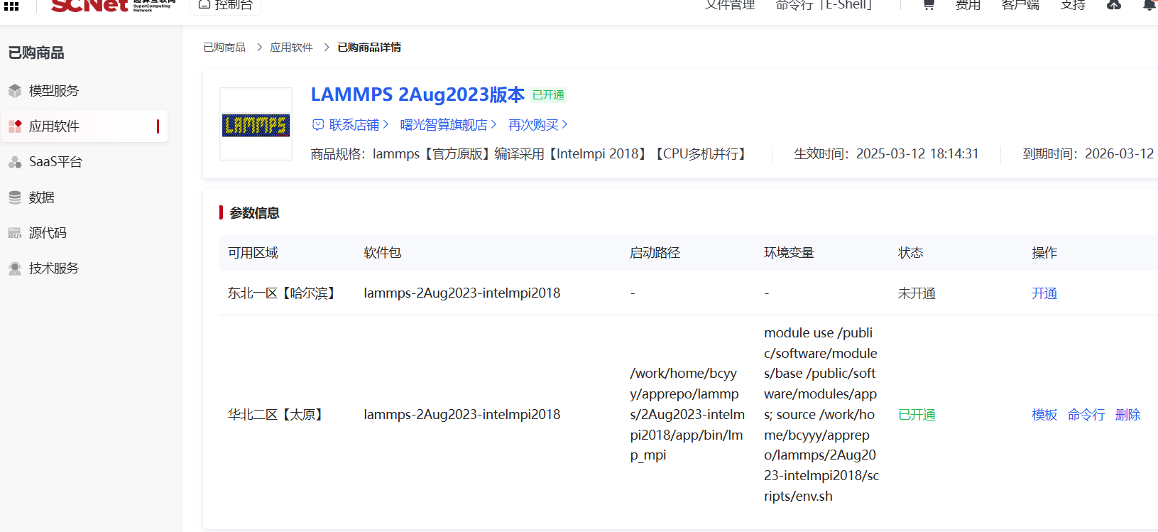
软件默认安装在家目录的apprepo下,环境变量默认放在软件scripts目录下的env.sh中。以下为典型的SLURM作业提交脚本示例:
#!/bin/bash
#SBATCH -J lammps_vacf  # 作业名称
#SBATCH -p normal       # 队列名称 (根据实际情况修改)
#SBATCH -N 2            # 节点数量
#SBATCH --ntasks-per-node=32 # 每节点核心数
module purge
source /path/to/your/apprepo/lammps/scripts/env.sh # 修改为你的实际路径

srun --mpi=pmi2 lmp_mpi -in in.VACF对于固态晶体,其原子的运动主要是围绕平衡位置的振动。VACF,即 C(t) = ⟨v(t) · v(0)⟩,描述了这种振动速度随时间的关联性。根据线性响应理论,VACF的傅里叶变换与系统的声子态密度(PDOS)直接相关:
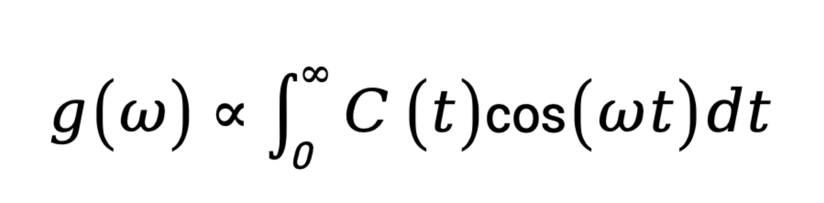
其中,g(ω)是频率为ω的振动模式的数量。因此,通过计算VACF,我们可以得到材料的振动谱,这是研究其热力学性质的基础。
本例以固态晶体硅作为研究对象,计算其在室温(300 K)下的VACF。
LAMMPS执行VACF计算仅需一个控制脚本。
# LAMMPS 计算速度自相关函数 (VACF) 脚本

# 基本变量设置
variable        simname index Si_vacf      # 模拟名称
variable        dt equal 0.0001            # 时间步长 (ps), 即 0.1 fs
variable        t equal 300                # 系统温度 (K)
log             log.${simname}.txt         # 日志文件

# 系统初始化
units           metal                      # 使用metal单位制
boundary        p p p                      # 周期性边界条件
timestep        ${dt}                      # 设置时间步长
atom_style      atomic                     # 原子模型类型

# 结构创建与势函数
lattice         diamond 5.43               # 定义晶体结构
region          box block 0.0 10.0 0.0 10.0 0.0 10.0 units lattice
create_box      1 box
create_atoms    1 region box

mass            1 28.0855                  # 硅原子质量
pair_style      tersoff                    # 选择Tersoff势
pair_coeff      * * SiC.tersoff Si         # 载入势参数

neighbor        1.0 bin                    # 近邻列表设置
neigh_modify    every 1 delay 0 check yes

# 热力学输出设置
thermo          100000
thermo_style    custom step temp press etotal

# 模拟过程解析
# 1. 能量最小化
min_style       cg
minimize        1e-25 1e-25 50000 100000

# 2. NPT系综平衡
#    将系统在300K, 0 Bar下弛豫,获得平衡的晶格常数和构型
fix             NPT1 all npt temp ${t} ${t} 0.1 iso 0.0 0.0 1.0
run             1000000
unfix           NPT1

# 3. NVE系综准备
#    切换到NVE系综,并用Langevin恒温器短暂运行以稳定温度
fix             NVE_run all nve
fix             thermostat all langevin ${t} ${t} 0.1 287859
run             100000
unfix           thermostat

# 4. VACF数据采集
#    在纯净的NVE系综下进行数据采集,保证能量守恒
compute         my_vacf all vacf
#    使用 fix ave/time 每步输出瞬时VACF值,用于后续后处理
fix             vacf_output all ave/time 1 1 1 c_my_vacf[1] c_my_vacf[2] c_my_vacf[3] c_my_vacf[4] file vacf_${simname}.dat format "%20.10f"
run             100000                      # 运行100000步进行采样

# 清理
unfix           NVE_run
unfix           vacf_output

print           "Simulation finished."
将上述脚本保存为 in.vacf,并确保 SiC.tersoff 势函数文件在同一目录下。通过 sbatch 命令提交作业即可开始计算。
LAMMPS 使用 fix ave/time 输出的 vacf.Si_vacf.dat 文件是原始的、未平均的数据,需要通过Python进行处理才能得到有意义的VACF曲线和声子谱。
# -*- coding: utf-8 -*-
import numpy as np
import matplotlib.pyplot as plt
from scipy.fft import rfft, rfftfreq

# --- User-defined Parameters ---
DATA_FILE = "vacf_Si_vacf.dat"  # LAMMPS output data file
TIMESTEP = 0.0001               # Timestep from the LAMMPS script (in ps)
SKIP_ROWS = 2                   # Number of header lines to skip in the data file
PDOS_X_LIMIT = 60             # Upper limit for the frequency axis in the PDOS plot (in THz)

# --- Data Loading ---
try:
    data = np.loadtxt(DATA_FILE, skiprows=SKIP_ROWS)
    print("Successfully loaded file '{0}', found {1} lines of data.".format(DATA_FILE, len(data)))
except FileNotFoundError:
    print("Error: File '{0}' not found. Please check the file name and path.".format(DATA_FILE))
    exit()
except Exception as e:
    print("An error occurred while reading the file: {0}".format(e))
    exit()

# --- Data Processing ---
if data.shape[1] < 5:
    print("Error: Data file has fewer than 5 columns. Cannot find the total VACF column.")
    exit()

# Use the 5th column (index 4) for the total VACF
vacf_raw = data[:, 4]

# Normalize the VACF so that C(0) = 1
if vacf_raw[0] == 0:
    print("Warning: The first value of VACF is zero. Skipping normalization.")
    vacf_normalized = vacf_raw
else:
    vacf_normalized = vacf_raw / vacf_raw[0]

# Create the time axis
num_steps = len(vacf_normalized)
time_axis = np.arange(num_steps) * TIMESTEP

# Calculate the Phonon Density of States (PDOS) via Fourier Transform
# Apply a Hanning window to reduce spectral leakage
window = np.hanning(num_steps)
pdos = np.abs(rfft(vacf_normalized * window))

# Calculate the corresponding frequency axis in THz
freq_axis_thz = rfftfreq(num_steps, d=TIMESTEP)

print("Data processing complete. Preparing to plot.")可视化VACF曲线和声子态密度是理解晶格动力学的关键。
# --- Visualization ---
fig, (ax1, ax2) = plt.subplots(2, 1, figsize=(8, 10))

# Plot 1: Velocity Autocorrelation Function (VACF)
ax1.plot(time_axis, vacf_normalized, lw=2, label='Normalized VACF')
ax1.set_xlabel('Time (ps)', fontsize=12)
ax1.set_ylabel('Normalized VACF', fontsize=12)
ax1.set_title('Velocity Autocorrelation Function (Solid Si @ 300 K)', fontsize=14)
ax1.axhline(0, color='gray', linestyle='--', lw=1)
ax1.grid(True, linestyle=':', alpha=0.6)
ax1.set_xlim(0, max(time_axis))
ax1.legend()

# Plot 2: Phonon Density of States (PDOS)
ax2.plot(freq_axis_thz, pdos, lw=2, color='orangered', label='PDOS')
ax2.set_xlabel('Frequency (THz)', fontsize=12)
ax2.set_ylabel('Phonon Density of States (a.u.)', fontsize=12)
ax2.set_title('Phonon Density of States (PDOS)', fontsize=14)
ax2.grid(True, linestyle=':', alpha=0.6)
ax2.set_xlim(0, PDOS_X_LIMIT)
ax2.legend()

# Final adjustments and saving the figure
plt.tight_layout()
plt.savefig('VACF_and_PDOS_analysis.png', dpi=300)
print("Plot saved as 'VACF_and_PDOS_analysis.png'")
plt.show()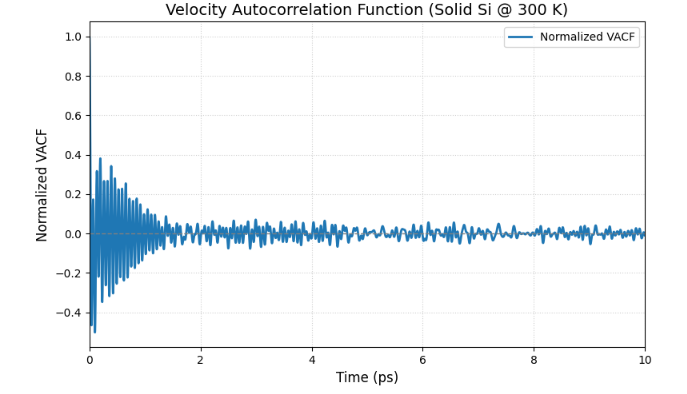
从VACF图中可以看到,曲线从1开始迅速衰减并呈现明显的振荡,这反映了原子在其晶格“笼子”中的周期性振动。固体的VACF曲线不会简单衰减至零,而是会持续振荡。
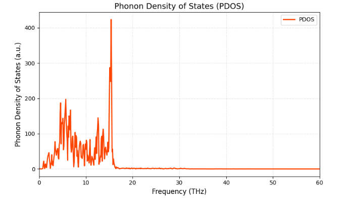
从PDOS图中,我们可以看到声子振动模式在不同频率上的分布。图中的峰值对应于声子谱中的特征峰,如横向声学(TA)、纵向声学(LA)、横向光学(TO)和纵向光学(LO)声子模。这些信息对于分析材料的热容、声速和热导率等性质至关重要。
本文详细介绍了在超算互联网使用LAMMPS计算固态晶体VACF的流程,并提供了使用Python进行数据处理、声子态密度计算和结果可视化的完整代码。通过这一流程,研究人员可以有效地分析晶格动力学行为和相关的热物理性质。
为了获得更精确的结果,建议采用更长的模拟时间和更优的统计平均方法,以减少统计噪声,获得更平滑的曲线和更清晰的PDOS。
参考资料: